Start with three questions: which frequency region is prominent, how long does it stay there, and what changes when another instrument enters? Read the axes and display settings before judging the shape. A peak is a place to investigate, not an instruction to cut.
What the graph actually shows
A real-time spectrum analyzer turns a short window of audio into a frequency display. In a magnitude plot such as Ableton Spectrum or the calculated figure below, frequency runs left to right and level runs vertically. A taller trace means a larger displayed spectral value at that frequency under the current settings—not automatically a problem or a measure of perceived loudness. A scrolling spectrogram uses a different map: do not transfer these axis meanings to Wave Candy without checking its display mode. Our calculated figure uses amplitude in dB relative to 1, not a loudness or room sound-pressure measurement.
Ableton describes Spectrum as a measurement tool that does not alter the signal. Its Block, Refresh and Avg controls change the trade-off between detail, speed and stability. FabFilter likewise exposes resolution, speed, range and tilt. Those settings change how the same audio looks, so a screenshot is not meaningful unless you know the analyzer configuration.
Set up the view in FL Studio or Ableton Live
FL Studio: read Wave Candy as a spectrogram
Insert Wave Candy on the Mixer track carrying the audio and select Spectrum mode. Its history moves across the horizontal time axis; frequency runs vertically and colour represents level. A brighter patch is not a higher frequency. Keep the mode fixed rather than letting Auto visual mode change it when you resize the window.
For this comparison, leave display Gain unchanged and match Max res, Scale, dB range and Natural weighting between views. These affect the displayed evidence. HOLD freezes the view; release it to follow the next phrase. None of those display choices substitutes for an audio-level adjustment.
To inspect an insert’s input and output, put one analyzer above it and another below it in the same serial effects stack. FL Studio processes Mixer slots from top to bottom. Avoid the selection-following Current track for this fixed comparison: selecting another track would change the source being inspected.
Ableton Live: compare two Spectrum devices
Place Spectrum before and after the target audio effect in a serial chain. On a MIDI track, both analyzers belong after the instrument. Match Block, Refresh, Avg, Channel and frequency scaling; use the same manual Range rather than separate Auto ranges. Spectrum does not process the audio. Unlike Wave Candy’s scrolling view, its ordinary graph puts frequency horizontally and dB vertically.
One-variable kick check: loop the same phrase, hold the analyzer settings fixed and change only the target effect. Compensate its output using the DAW trim-placement workflow, then listen for attack, tail texture and space around the bass. A brighter spectrogram or taller trace can reflect extra level, not a better mix. Parallel racks and sends need separate routing checks; this example describes one serial path.
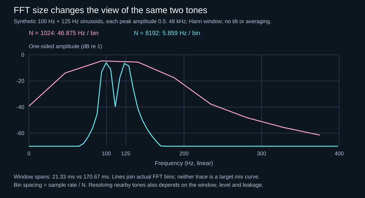
The two-tone graph above is our declared calculation, not a Wave Candy or Spectrum screenshot. Neither host view is promised to reproduce its exact curve: compare the settings and normalization, and use the reproduction conditions below when checking the mathematics.
Read shape, movement and relationships
Do not chase every narrow peak. First read the large-scale shape: where the low-end mass sits, how energy falls toward the top, and whether one broad region dominates. Then watch movement. For example, kick-related low energy may pulse while a sustained rumble remains between hits. The trace alone cannot identify an instrument or distinguish a fundamental from a stronger harmonic; audition the sources.
The most useful information is often relational. Put the kick and bass on separate analyzers or compare them through an external spectrum. If both remain strong in the same low band at the same moment, masking is possible. FabFilter explicitly calls collision detection an indication rather than exact science. Listen while lowering the competing part; improved audibility is a useful clue, not a diagnosis from the trace alone. A polarity comparison answers a different question about summing.
The controls change the evidence
- Resolution or block size: more samples improve low-frequency detail but make the display react more slowly. Use higher resolution to investigate a kick fundamental; use a faster view to follow transients.
- Refresh versus decay: refresh changes how often the display updates; a speed/decay control changes how long old energy remains visible. They are not the same as the FFT window length. Check what your analyzer’s control actually does.
- Averaging: more averaging smooths short changes into a stable trend. Ableton notes that this is closer to how we perceive a spectrum over time, but it can hide a brief spike.
- Tilt: a tilted display compensates visually for the natural downward slope common in music. FabFilter’s default is 4.5 dB per octave around 1 kHz, but that is a viewing choice—not a target curve for every record.
- Pre versus post: pre-EQ shows the input; post-EQ shows the result. Display both when checking whether a move changed the intended area or created a new imbalance.
- Channel and scale: keep left/right/stereo selection and vertical range fixed. Ableton Spectrum can automatically rescale its view; switch to a fixed range when comparing heights. Do not assume two analyzers calculate a combined-channel trace in the same way.
- Freeze or maximum hold: useful for catching intermittent peaks, provided you reset it between comparisons.
Two matching spectra can still sum differently
A magnitude spectrum omits phase. Inverting an isolated signal changes its sign but leaves its magnitude spectrum unchanged. Adding that signal to another source can nevertheless change the summed level. A red collision area, two overlapping curves or matching solo spectra therefore cannot establish cancellation. Use a controlled pair test and the phase and polarity guide, then return to the full phrase.
A same-spectrum, different-sum experiment
- In a saved test session at a low monitoring level, duplicate one mono audio clip onto two identically routed tracks. Keep timing and gain equal, with no random processing or bus dynamics. Watch the common bus, not only the two solo tracks.
- Compare one track with both copies. Their coherent sum has twice the amplitude, approximately +6.02 dB before any normalization; leave enough headroom. This is a calculated identity for exact copies, not a target for kick/bass mixing.
- Invert one copy. Ideal equal copies cancel at the bus, while their separate magnitude spectra remain identical. Imperfect matching, differing routing or processing can leave a residual. Restore the polarity afterward.
Independent kick and bass parts are not duplicate clips. The lesson is to distinguish the source spectra from their sum—not to seek a null or a fixed gain increase in a real arrangement. If the sound stays present but becomes hard to hear, follow the masking, cancellation and ducking diagnosis before deciding on EQ.
A four-pass hard-techno check
- Calibrate the view. Loop the loudest representative drop. Use one analyzer configuration throughout the comparison and level-match references before judging their shapes.
- Solo to identify, then return to context. Find the kick’s fundamental and tail while soloed. Bring the rumble or bass back and listen for loss of punch, pitch blur or a tail that never clears.
- Search suspicious peaks with your ears. If a narrow line persists, sweep or band-solo only to locate it. Reduce it temporarily, level-match and ask whether the mix becomes clearer. If not, undo the move.
- Verify outside the graph. Check quietly, in mono, on headphones and on a small speaker. A sub-heavy trace may simply describe a club-focused balance; it becomes a fault when translation or headroom suffers.
Resolution is more than the number of drawn points
FFT bin spacing is sample rate divided by block size. At 48 kHz, 4096 samples span about 85.33 ms with 11.72 Hz between bins. This is a calculation, not a recommended setting. A longer block gathers more time to distinguish nearby low tones. Window shape, leakage and relative levels also affect resolution; interpolation or zero-padding can draw a smoother curve without creating new information.
A window changes the trade-off between separating close components and seeing weaker components beside strong ones. NI explains this through main-lobe width and side-lobe leakage. A clean-looking curve can conceal that trade-off; keep the window type fixed when testing block size.
Reproduce the two-tone example
- At a safe monitoring level, sum sine test tones at 100 Hz and 125 Hz in a 48 kHz session. Each tone in our calculation has peak amplitude 0.5. These define the illustrated test, not recommended mix settings.
- Compare 1024- and 8192-sample blocks using the same Hann window, level, vertical scale and no tilt or averaging. A different analyzer’s normalization may change the displayed heights.
- Watch whether two nearby components become distinguishable. Do not interpret wider skirts around a line as newly generated distortion: they can come from the finite analysis window.
- Return to a kick/bass loop and ask what the extra detail helps you identify. If it does not explain an audible problem, do not add an EQ move merely to tidy the picture.
Finding a kick fundamental without guessing
A pitched kick often creates a low-frequency peak plus a ladder of harmonics. Hovering over the analyzer can report frequency or note name, and FabFilter’s Spectrum Grab can freeze and identify prominent peaks. Treat the label as a clue: the tallest peak can be a harmonic, and the fundamental can be weak or absent. Distorted kicks change pitch through the tail, so one static note cannot describe the entire event.
As a starting process, shorten the loop, raise analyzer resolution and compare the attack with the later tail. Listen for whether the perceived pitch agrees with the trace. If the bass occupies the same area, check arrangement, envelope, tuning and timing before reaching automatically for a deep EQ cut.
“Higher resolution” does not isolate a shorter moment. At 48 kHz, an 8192-sample block spans about 170.67 ms; a requested 30 ms attack view cannot fit inside that block without including surrounding material or padding. These are calculated example durations, not recommended settings. A falling kick pitch can spread across several frequencies during one window. Compare a faster view for movement with a longer view of a relatively stable tail, and use the sampler playback checks before assuming a shorter MIDI note changes the audio.
Excess sub versus intentional pressure
Energy below the useful musical low end can consume peak headroom without creating proportionate impact on many systems. But there is no universal high-pass frequency. A hard-techno kick, a pitched hardcore tail and a rumble all need different treatment.
Test a filter at a conservative starting point, bypass it at matched loudness and listen for body loss, cleaner limiting and improved kick/bass separation. Move the cutoff only while the full arrangement plays. The analyzer confirms what changed; the monitoring chain and reference material decide whether the change helped.
Three traps that create worse mixes
- Flat-line mixing: forcing every band to the same height ignores musical balance, analyzer tilt and human hearing.
- Peak hunting: cutting every visible line removes resonant identity and turns a powerful kick into noise without focus.
- Unmatched references: the louder master usually looks fuller. Level-match and compare similar sections before drawing conclusions.
The analyzer tells you where to ask a question. The speakers tell you whether the answer works.
What the sources emphasize — and our conclusion
Ableton separates block length, display refresh, averaging and channel selection. FabFilter focuses on adjustable resolution, visual tilt and external-spectrum comparison. NI explains why window shape trades separation of nearby components against leakage from strong ones. These descriptions solve different parts of the same measurement problem; none makes a musical decision for you.
JDMEET’s working rule: first change only the display and notice what moves while the audio remains unchanged. Then change one audible variable, keep the analyzer configuration fixed and judge the complete phrase. Only a change that helps the named musical problem earns a place in the mix.